Frequently Asked Questions
Below are answers to common questions about using agtools for working with assembly graphs.
Q1. What is agtools?
agtools provides a command-line interface for manipulating assembly graphs, as well as a Python package interface for exploring assembly graphs in your own software. You can refer to the following resources to get an overview of agtools' capabilities.
Q2. Why would I need agtools?
Assembly graphs are gaining popularity, particularly in the metagenomics domain, as they contain valuable connectivity information about assembled sequences. This information can be extremely useful for downstream applications such as:
- Metagenomic binning - GraphBin, MetaCoAG, GraphMB
- Resolving bacterial strains - STRONG
- Resolving viral strains - VStrains, Phables
- Identifying plasmids - GraphPlas
- Sequence classification - 3CAC, 4CAC
Many applications require a programmatic and modular way to explore and manipulate assembly graphs. However, no standardised solution currently exists, and developers often resort to writing custom, one-off code. agtools bridges this gap by offering a reusable and extensible toolkit for working with assembly graphs in a consistent and accessible manner.
Q3. What assemblers are supported for contig graph generation?
Currently, agtools supports contig graphs generated by the following assemblers with tested versions, each of which introduces certain assembler-specific nuances:
- SPAdes (and metaSPAdes) - 3.15.5
- MEGAHIT - 1.2.9
- Flye (and metaFlye) - 2.9.6-b1802
- myloasm - 0.1.0
If you want to load a contig-level assembly graph from another assembler that follows the standard GFA format, you can use the from_gfa function from the UnitigGraph class.
If you have a contig-level assembly graph from an assembler that is not listed above and has assembler-specific nuances, please submit a feature request via agtools Issues.
Q4. How are edges counted in the assembly graph?
Below is an example assembly graph.
S   1   TTCGCTGCGCTCGCTTCGCTTT  DP:f:5
S   2   TGCCGTCGTCGCTGTGCA  DP:f:4
S   3   TGCCTGAATCGCCTA DP:f:1
S   4   GCTCGGCTCG  DP:f:4
S   5   CGAACCAT    DP:f:2
S   6   TACTTGT DP:f:1
S   7   GCCTT   DP:f:2
S   8   ATCT    DP:f:1
S   9   GC  DP:f:1
S   10  T   DP:f:1
L   1   +   4   +   0M
L   4   -   1   -   0M
L   1   +   5   -   0M
L   5   +   1   -   0M
L   2   +   1   +   0M
L   1   -   2   -   0M
L   3   -   1   +   0M
L   1   -   3   +   0M
L   4   +   7   -   0M
L   7   +   4   -   0M
L   4   +   8   +   0M
L   8   -   4   -   0M
L   6   -   5   -   0M
L   5   +   6   +   0M
L   6   +   6   -   0M
L   7   -   9   +   0M
L   9   -   7   +   0M
L   8   +   10  -   0M
L   10  +   8   -   0M
L   9   +   7   +   0M
L   7   -   9   -   0M
If you visualise this graph using Bandage, it will appear as follows.
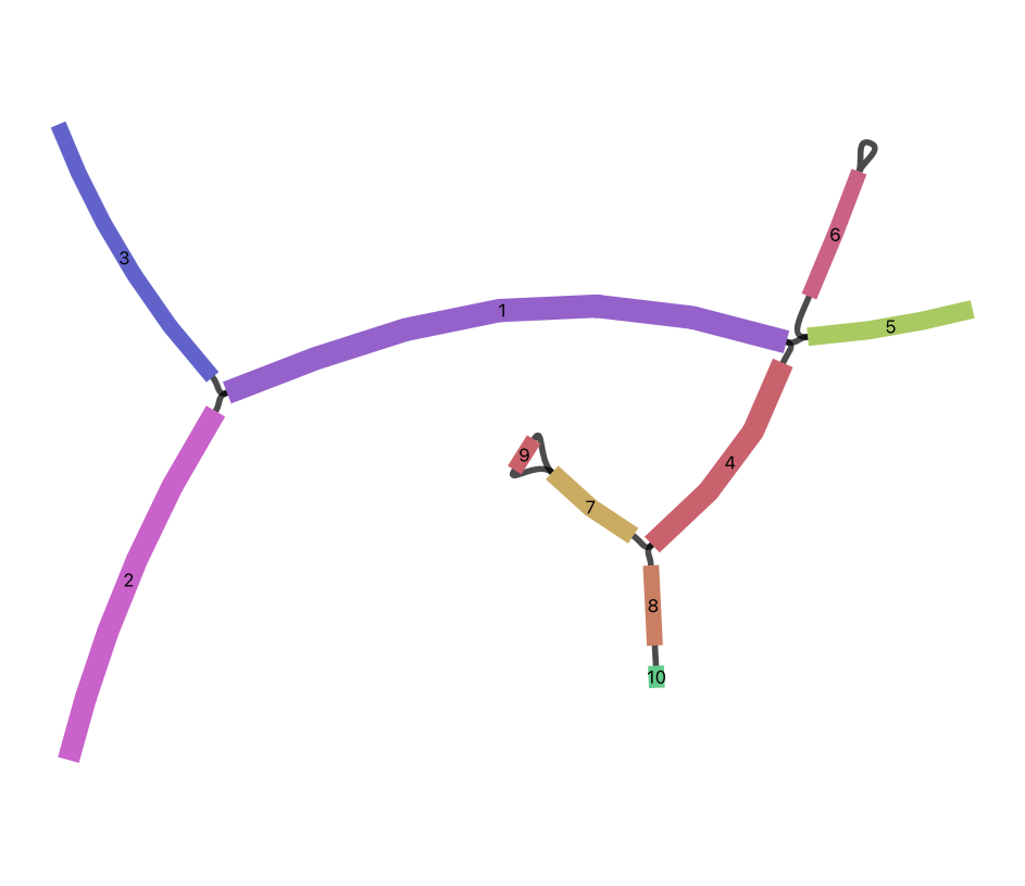
Let’s load the GFA file and query the edges and links.
>>> from agtools.core.unitig_graph import UnitigGraph
>>> ug = UnitigGraph.from_gfa("assembly_graph.gfa")
>>> ug.ecount
9
>>> ug.lcount
21
ug.lcount reports the number of lines in the GFA file that begin with the L tag (21 in this case).
If you look at the Bandage visualisation, there are 11 links: segment 9 has two links with different orientations, and segment 6 has a self-loop. However, ** agtools does not represent a directed assembly graph**. Instead, it represents only the connectivity between segments.
Multiple edges and self-loops are removed to simplify the graph. This is why ug.ecount differs from the number of L records in the GFA file.
The resulting simplified graph is shown below.
